ᱠᱮᱞᱤ ᱠᱨᱟᱭᱴᱮᱨᱤᱭᱚᱱ ᱟᱨ ᱨᱩᱞᱮᱴ
ᱠᱮᱞᱤ ᱠᱨᱟᱭᱴᱮᱨᱤᱭᱚᱱ ᱫᱚ ᱵᱟᱲᱛᱤ ᱢᱮᱱᱟᱜ ᱵᱟᱡᱤ ᱞᱟᱜᱟᱣᱤᱡ ᱮ ᱢᱮᱱᱟᱜ-ᱟ ᱡᱮ ᱛᱤᱱᱟᱹᱜ ᱵᱟᱡᱤ ᱴᱟᱠᱟ ᱞᱟᱜᱟᱣ ᱞᱟᱹᱠᱛᱤ᱾ ᱨᱩᱞᱮᱴ ᱞᱟᱹᱜᱤᱫ ᱚᱱᱟ ᱨᱮᱭᱟᱜ ᱛᱮᱞᱟ ᱥᱟᱯᱷᱟ: ᱪᱮᱫ ᱦᱚᱸ ᱵᱟᱝ᱾

ᱠᱮᱞᱤ ᱵᱟᱡᱤ ᱴᱟᱠᱟ = ᱵᱟᱲᱛᱤ / ᱚᱰᱥ᱾ ᱱᱮᱜᱮᱴᱤᱵᱷ ᱵᱟᱲᱛᱤ ᱨᱮ ᱯᱷᱚᱨᱢᱩᱞᱟ ᱫᱚ ᱱᱮᱜᱮᱴᱤᱵᱷ ᱦᱟᱹᱴᱤᱧ ᱮᱢᱟ, ᱚᱱᱟ ᱨᱮᱭᱟᱜ ᱢᱟᱱᱮ: ᱵᱟᱡᱤ ᱟᱞᱚᱢ ᱞᱟᱜᱟᱣᱟ᱾ ᱱᱚᱶᱟ ᱠᱨᱟᱭᱴᱮᱨᱤᱭᱚᱱ ᱫᱚ ᱱᱤᱛ ᱦᱚᱸ ᱵᱩᱡᱷᱟᱹᱣ ᱞᱟᱹᱜᱤᱫ ᱠᱟᱹᱢᱤ ᱨᱮ ᱦᱟᱜᱩᱜ-ᱟ ᱡᱮ ᱵᱟᱭᱟᱥ ᱠᱷᱮᱞᱚᱸᱰ ᱠᱚ ᱫᱚ ᱪᱮᱫᱟᱜ ᱚᱱᱟ ᱞᱮᱠᱟ ᱵᱟᱡᱤ ᱢᱟᱯ ᱠᱚ ᱵᱟᱪᱷᱟᱣ ᱞᱮᱫᱟ, ᱟᱨ ᱮᱴᱟᱜ ᱡᱚᱛᱚ ᱦᱚᱲ ᱫᱚ ᱪᱮᱫᱟᱜ ᱵᱟᱡᱮᱴ ᱞᱮᱠᱷᱟ ᱛᱮ ᱵᱟᱡᱤ ᱢᱟᱯ ᱵᱟᱪᱷᱟᱣ ᱞᱟᱹᱠᱛᱤᱭᱟ᱾
ᱠᱨᱟᱭᱴᱮᱨᱤᱭᱚᱱ
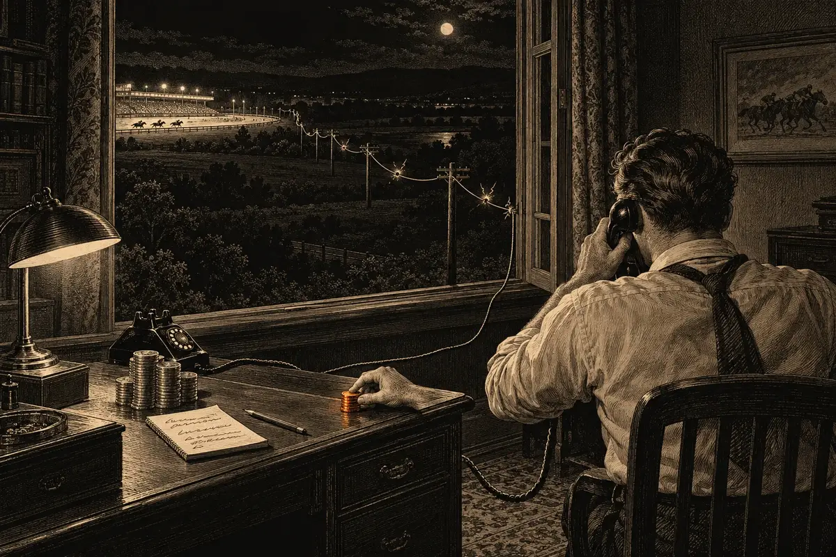
John Kelly (1956) asked how a gambler with a known edge should size bets to maximize long-run growth of the bankrollᱴᱟᱠᱟᱠᱷᱮᱞ ᱯᱩᱸᱡᱤᱠᱷᱮᱞ ᱞᱟᱹᱜᱤᱫ ᱟᱞᱟᱜ ᱫᱚᱦᱚ ᱟᱠᱟᱱ ᱡᱚᱛᱚ ᱴᱟᱠᱟ᱾ ᱠᱷᱮᱞ ᱯᱩᱸᱡᱤ ᱥᱟᱢᱵᱷᱟᱞ ᱫᱚ ᱢᱮᱱᱮᱛ ᱢᱤᱫ ᱵᱟᱡᱤ ᱟᱨ ᱢᱤᱫ ᱥᱮᱥᱚᱱ ᱨᱮ ᱚᱱᱟ ᱠᱷᱚᱱ ᱛᱤᱱᱟᱹᱜ ᱡᱚᱠᱷᱤᱢ ᱨᱮ ᱫᱚᱦᱚᱭ ᱚᱱᱟ ᱴᱷᱟᱹᱣᱠᱟᱹ᱾ᱯᱩᱨᱟᱹ ᱯᱟᱲᱦᱟᱣ →. The answer, for a bet paying b to 1 with win probabilityᱜᱚᱱᱤᱛᱥᱚᱢᱵᱷᱟᱵᱱᱟᱢᱤᱫ ᱨᱮᱡᱟᱞᱴ ᱨᱮᱭᱟᱜ ᱥᱚᱢᱵᱷᱟᱵᱱᱟ, 0 ᱠᱷᱚᱱ 1 ᱟᱨᱵᱟᱝ 0% ᱠᱷᱚᱱ 100%᱾ ᱢᱤᱫ ᱮᱞ: 1/37 = 2.70%᱾ᱯᱩᱨᱟᱹ ᱯᱟᱲᱦᱟᱣ → p and loss probability q = 1 − p, is to stake the fraction f* = (bp − q) / b of the bankroll. Positive f* means bet that fraction; zero or negative means do not bet. Kelly worked at Bell Labs, and his paper, “A new interpretation of information rate”, set the problem in Claude Shannon’s theory of information: a gambler who gets tips over a noisy line, at fair odds, can grow the bankroll at best at the rate the line carries information. This is a growth objective under a probability model, not a promise to finish ahead after a particular number of bets. A spending limit, finite deadline or payoutᱴᱟᱠᱟᱵᱷᱩᱜᱛᱟᱱᱡᱤᱛ ᱵᱟᱡᱤ ᱪᱮᱫ ᱨᱩᱣᱟᱹᱲᱟ, ᱨᱩᱣᱟᱹᱲ ᱵᱟᱡᱤ ᱴᱟᱠᱟ ᱪᱮᱛᱟᱱ “X ᱨᱮ 1” ᱞᱮᱠᱟ ᱨᱚᱲᱚᱜ-ᱟ᱾ᱯᱩᱨᱟᱹ ᱯᱟᱲᱦᱟᱣ → cap changes the decision problem.
ᱨᱩᱞᱮᱴ ᱨᱮ ᱠᱮᱞᱤ ᱵᱟᱡᱤ
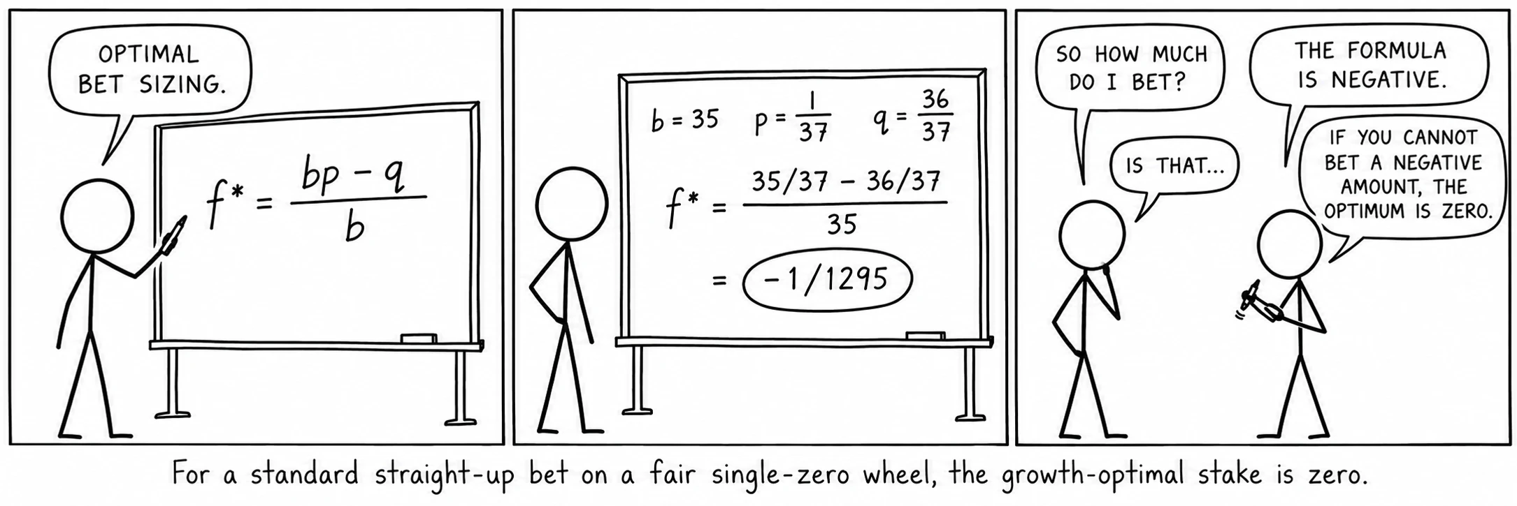
For redᱵᱟᱡᱤᱟᱨᱟᱜ18 ᱟᱨᱟᱜ ᱮᱞ ᱨᱮ ᱥᱚᱢᱟᱱ ᱴᱟᱠᱟ ᱵᱟᱡᱤ᱾ ᱯᱷᱨᱮᱧᱪ ᱨᱮ: ᱨᱩᱡᱽ᱾ᱯᱩᱨᱟᱹ ᱯᱟᱲᱦᱟᱣ →: b = 1, p = 18/37, q = 19/37; f* = (18/37 − 19/37)/1 = −1/37. For a straight upᱵᱟᱡᱤᱥᱴᱨᱮᱴ ᱚᱯᱢᱤᱫ ᱮᱞ, ᱵᱷᱩᱜᱛᱟᱱ 35:1᱾ᱯᱩᱨᱟᱹ ᱯᱟᱲᱦᱟᱣ →: b = 35, p = 1/37, q = 36/37; f* = (35/37 − 36/37)/35 = −1/1295. Every standard bet gives a negative Kelly fraction, because every bet has a negative edge, and the growth-optimal stake is zero. Kelly betting on roulette is a formal way of saying what the house-edge page says: no positive stake maximizes expected logarithmic growth when the bet has negative expectation. A particular session can still end in profit. La partageᱱᱤᱭᱚᱢᱞᱟ ᱯᱟᱨᱛᱟᱡᱽᱯᱷᱨᱮᱧᱪ ᱱᱤᱭᱚᱢ: ᱡᱤᱨᱚ ᱦᱤᱡᱩᱜ ᱞᱮᱠᱷᱟᱱ ᱥᱚᱢᱟᱱ ᱴᱟᱠᱟ ᱵᱟᱡᱤ ᱨᱮᱭᱟᱜ ᱟᱫᱷᱟ ᱨᱩᱣᱟᱹᱲᱚᱜ-ᱟ᱾ ᱚᱱᱟ ᱵᱟᱡᱤ ᱠᱚ ᱨᱮ ᱠᱮᱥᱤᱱᱳ ᱵᱟᱲᱛᱤ ᱟᱫᱷᱟ, 1.35% ᱦᱩᱭᱩᱜ-ᱟ᱾ᱯᱩᱨᱟᱹ ᱯᱟᱲᱦᱟᱣ → needs a separate three-outcome calculation: a win, a full loss or a half-loss on zeroᱪᱟᱠᱟᱡᱤᱨᱚᱢᱤᱫᱜᱮ ᱦᱟᱹᱨᱭᱟᱹᱲ ᱠᱷᱟᱱᱟ ᱡᱟᱦᱟᱸ ᱥᱚᱢᱟᱱ ᱴᱟᱠᱟ, ᱰᱚᱡᱮᱱ ᱟᱨᱵᱟᱝ ᱠᱚᱞᱚᱢ ᱵᱟᱡᱤ ᱵᱟᱭ ᱠᱚᱵᱷᱟᱨᱟ; ᱠᱮᱥᱤᱱᱳ ᱵᱟᱲᱛᱤ ᱨᱮᱭᱟᱜ ᱢᱩᱞ᱾ ᱮᱴᱟᱜ ᱧᱩᱛᱩᱢ: ᱥᱤᱝᱜᱚᱞ ᱡᱤᱨᱚ, 0᱾ᱯᱩᱨᱟᱹ ᱯᱟᱲᱦᱟᱣ →. Its expected log growth also falls as the stake increases from zero.
ᱚᱠᱟ ᱨᱮ ᱠᱮᱞᱤ ᱫᱚ ᱠᱟᱹᱢᱤ ᱞᱮᱫᱟ
Suppose a pocketᱥᱟᱡ ᱥᱟᱢᱟᱱᱠᱷᱟᱱᱟᱨᱚᱴᱚᱨ ᱨᱮᱭᱟᱜ 37 ᱮᱞ ᱚᱞ ᱠᱷᱟᱱᱟ ᱠᱷᱚᱱ ᱢᱤᱫ᱾ ᱮᱴᱟᱜ ᱧᱩᱛᱩᱢ: ᱥᱞᱚᱴ, ᱠᱟᱯ᱾ᱯᱩᱨᱟᱹ ᱯᱟᱲᱦᱟᱣ → really has a stable, known probability of 1 in 30 and pays 35 to 1. The Kelly fraction is 0.57%: about $57 from a $10,000 bankroll. Under independent spinsᱜᱚᱱᱤᱛᱟᱡᱟᱫ ᱜᱷᱩᱨᱟᱹᱣᱢᱟᱨᱮ ᱪᱮᱫ ᱦᱚᱸ ᱦᱩᱭ ᱠᱷᱟᱱ ᱦᱚᱸ ᱡᱚᱛᱚ ᱜᱷᱩᱨᱟᱹᱣ ᱨᱮ ᱥᱚᱢᱵᱷᱟᱵᱱᱟ ᱢᱤᱫ ᱞᱮᱠᱟ ᱜᱮ᱾ ᱱᱚᱶᱟ ᱥᱟᱭᱤᱴ ᱨᱮᱭᱟᱜ ᱡᱚᱛᱚ ᱦᱤᱥᱟᱹᱵ ᱨᱮᱭᱟᱜ ᱵᱮᱥ᱾ᱯᱩᱨᱟᱹ ᱯᱟᱲᱦᱟᱣ → and exact fractional staking, the geometric growth factor over 1,000 spins is about 1.7. Expected bankroll grows faster because rare large wins pull up the average. These are model calculations, not evidence that any named historical player used Kelly or achieved this result.
ᱥᱟᱫᱷᱟᱨᱚᱬ ᱟᱨ ᱟᱣᱥᱚᱛ
The gap between the typical bankroll and the average one is wide. Take a pocket that hits 1 time in 25, a hypothetical edge of 44% per unitᱴᱟᱠᱟᱭᱩᱱᱤᱴᱢᱤᱫ ᱥᱤᱥᱴᱮᱢ ᱟᱨᱵᱟᱝ ᱠᱷᱮᱞᱚᱸᱰ ᱵᱮᱵᱷᱟᱨ ᱵᱮᱥ ᱵᱟᱡᱤ ᱴᱟᱠᱟ᱾ ᱯᱨᱚᱜᱽᱨᱮᱥᱚᱱ ᱠᱚ ᱭᱩᱱᱤᱴ ᱛᱮ ᱵᱩᱡᱷᱟᱹᱣᱚᱜ-ᱟ ᱡᱮᱢᱚᱱ ᱡᱟᱦᱟᱸᱱ ᱴᱮᱵᱩᱞ ᱨᱮ ᱞᱟᱹᱜᱩ ᱦᱩᱭᱩᱜ-ᱟ᱾ᱯᱩᱨᱟᱹ ᱯᱟᱲᱦᱟᱣ → staked. Kelly stakes 1.26% of the bankroll on it. After 1,000 spins the typical bankroll has grown about 11.5 times, while the average, pulled up by a few very lucky runs, has grown about 249 times. Betting more than Kelly raises the average and lowers the typical result: at twice the Kelly stake the typical bankroll only doubles, and by two and a half times the Kelly stake it shrinks, although every bet still carries a 44% edge. In this example, half-Kelly retains about 78% of the expected log growth. This fraction depends on the probabilities and payout.
ᱵᱟᱲᱛᱤ ᱫᱚ ᱟᱸᱫᱟᱡᱽ ᱜᱮ ᱠᱷᱟᱱ
Kelly uses the true probabilities, but a player usually has only estimates. Selecting the busiest pocket from a past record creates a selection problem: even a fair wheel has a busiest pocket. Its observed rate can overstate its future probability. Choosing the stake from that same record compounds the error. An independent follow-up sample helps test a proposed bias (see How to Detect Roulette Wheel Bias). Reducing the calculated fraction reduces exposure, but cannot turn a false edge into a real one.
ᱵᱟᱲᱛᱤ ᱢᱮᱱᱟᱜ ᱦᱚᱲ
Haghani and Dewey (2016) studied 61 participants given $25 and 30 minutes to bet on a simulated coin with a disclosed 60% chance of heads. The payout cap was $250; its value was revealed when a proposed winning bet would reach it. Their reported 21% success category included balances of at least $200, while the 28% “bust” category meant less than $2, not necessarily zero. Eighteen participants bet their entire balance on one flip. The uncapped Kelly fraction is 20%, but the cap and deadline change the optimization problem. The experiment illustrates how stake choices matter even with a known advantage; it does not establish one best strategy for every objective.
ᱚᱱᱟ ᱵᱚᱫᱚᱞ ᱛᱮ ᱪᱮᱫ ᱵᱮᱵᱷᱟᱨ ᱦᱩᱭᱩᱜ-ᱟ
ᱵᱟᱲᱛᱤ ᱵᱟᱹᱱᱩᱜ ᱠᱷᱟᱱ, ᱵᱟᱡᱤ ᱢᱟᱯ ᱫᱚ ᱵᱟᱡᱮᱴ ᱨᱮᱭᱟᱜ ᱠᱩᱠᱞᱤ ᱠᱟᱱᱟ, ᱵᱟᱹᱲᱛᱤ ᱨᱮᱭᱟᱜ ᱫᱚ ᱵᱟᱝ: ᱵᱟᱡᱤ ᱴᱟᱠᱟ = ᱢᱤᱫ ᱜᱷᱩᱨᱟᱹᱣ ᱨᱮ ᱟᱯᱮ ᱛᱤᱱᱟᱹᱜ ᱠᱷᱚᱨᱚᱪ ᱥᱟᱱᱟᱭ ᱠᱟᱱᱟ ᱯᱮ, ᱡᱟᱦᱟᱸ ᱫᱚ ᱢᱤᱫ ᱜᱷᱟᱸᱴᱟ ᱨᱮᱭᱟᱜ ᱵᱟᱡᱮᱴ ᱟᱨ ᱴᱮᱵᱩᱞ ᱨᱮᱭᱟᱜ ᱞᱚᱜᱚᱱ ᱠᱷᱚᱱ ᱦᱤᱥᱟᱹᱵ ᱦᱩᱭᱩᱜ-ᱟ (ᱨᱩᱞᱮᱴ ᱠᱷᱮᱞ ᱯᱩᱸᱡᱤ ᱥᱟᱢᱵᱷᱟᱞ ᱥᱟᱦᱴᱟ)᱾ ᱥᱟᱫᱷᱟᱨᱚᱬ ᱠᱷᱮᱞᱚᱸᱰ ᱞᱟᱹᱜᱤᱫ ᱠᱮᱞᱤ ᱨᱮᱭᱟᱜ ᱮᱢ ᱫᱚ ᱚᱱᱟ ᱨᱮᱭᱟᱜ ᱥᱟᱯᱷᱟ ᱛᱮᱞᱟ: ᱡᱤᱨᱚ᱾ ᱡᱤᱨᱚ ᱠᱷᱚᱱ ᱪᱮᱛᱟᱱ ᱡᱟᱦᱟᱸ ᱵᱟᱡᱤ ᱟᱯᱮ ᱞᱟᱜᱟᱣᱟ ᱯᱮ, ᱚᱱᱟ ᱫᱚ ᱠᱷᱮᱞ ᱨᱮᱭᱟᱜ ᱫᱟᱢ ᱠᱟᱱᱟ, ᱟᱯᱮ ᱛᱮ ᱵᱟᱪᱷᱟᱣ ᱟᱠᱟᱱ, ᱡᱟᱦᱟᱱᱟᱜ ᱯᱷᱚᱨᱢᱩᱞᱟ ᱛᱮ ᱵᱮᱥ ᱵᱮᱱᱟᱣ ᱟᱠᱟᱱ ᱫᱚ ᱵᱟᱝ᱾
ᱦᱟᱹᱴᱤᱧ ᱠᱮᱞᱤ ᱟᱨ “ᱴᱟᱠᱟ ᱥᱟᱢᱵᱷᱟᱞ” ᱵᱟᱵᱚᱛ ᱢᱤᱫ ᱠᱟᱛᱷᱟ
Betting a fixed percentage of the current bankroll is proportional staking: the stake rises after wins and falls after losses. Flat bettingᱥᱴᱨᱮᱴᱮᱡᱤᱢᱤᱫ ᱞᱮᱠᱟᱱ ᱵᱟᱡᱤᱡᱚᱛᱚ ᱜᱷᱩᱨᱟᱹᱣ ᱨᱮ ᱢᱤᱫ ᱞᱮᱠᱟᱱ ᱴᱟᱠᱟ ᱵᱟᱡᱤ᱾ ᱡᱚᱛᱚ ᱯᱨᱚᱜᱽᱨᱮᱥᱚᱱ ᱱᱚᱶᱟ ᱥᱟᱶ ᱛᱩᱞᱟᱹᱣᱚᱜ-ᱟ᱾ᱯᱩᱨᱟᱹ ᱯᱟᱲᱦᱟᱣ → instead keeps the cash stake fixed. Neither creates an edge on ordinary roulette. With infinitely divisible stakes and a fraction below 100%, proportional staking never reaches exactly zero in finitely many losses, but the balance can become arbitrarily small. Real table minimums can prevent further play much sooner. The growth-optimal fraction remains zero.
ᱯᱷᱚᱨᱢᱩᱞᱟ
ᱠᱩᱠᱞᱤ ᱠᱚ
Only when the actual probabilities, payouts and conditions give a credible positive advantage. Standard bets on an unbiased wheel have no such advantage.
Using half the calculated fraction reduces exposure to errors in the estimated edge. The familiar three-quarters-growth rule is an approximation for small advantages, not a universal identity. It does not protect against an edge that does not exist.
ᱵᱟᱝ᱾ ᱠᱮᱞᱤ ᱫᱚ ᱵᱟᱲᱛᱤ ᱛᱟᱦᱮᱸᱱ ᱠᱷᱟᱱ ᱵᱟᱹᱲᱛᱤ ᱮ ᱵᱮᱥᱟᱭᱟ᱾ ᱠᱷᱮᱞ ᱯᱩᱸᱡᱤ ᱥᱟᱢᱵᱷᱟᱞ ᱫᱚ ᱵᱟᱲᱛᱤ ᱵᱟᱹᱱᱩᱜ ᱠᱷᱟᱱ ᱠᱷᱚᱨᱚᱪ ᱥᱟᱢᱵᱷᱟᱞᱟ᱾
ᱜᱚᱱᱤᱛ ᱥᱟᱶ ᱨᱟᱹᱥᱠᱟᱹ
ᱱᱚᱶᱟ ᱠᱚ ᱯᱩᱭᱞᱩ ᱟᱯᱮ ᱛᱮ ᱠᱩᱨᱩᱢᱩᱴᱩ ᱯᱮ᱾ ᱢᱤᱫ ᱢᱤᱫ ᱥᱚᱢᱟᱫᱷᱟᱱ ᱫᱚ ᱩᱠᱩ ᱢᱮᱱᱟᱜ-ᱟ; ᱛᱮᱭᱟᱨ ᱦᱩᱭ ᱠᱟᱛᱮ ᱡᱷᱤᱡᱽ ᱯᱮ᱾
Suppose a hypothetical bet on one number has a known 44% edge under standard payoutsᱴᱟᱠᱟᱵᱷᱩᱜᱛᱟᱱᱡᱤᱛ ᱵᱟᱡᱤ ᱪᱮᱫ ᱨᱩᱣᱟᱹᱲᱟ, ᱨᱩᱣᱟᱹᱲ ᱵᱟᱡᱤ ᱴᱟᱠᱟ ᱪᱮᱛᱟᱱ “X ᱨᱮ 1” ᱞᱮᱠᱟ ᱨᱚᱲᱚᱜ-ᱟ᱾ᱯᱩᱨᱟᱹ ᱯᱟᱲᱦᱟᱣ → and independent spinsᱜᱚᱱᱤᱛᱟᱡᱟᱫ ᱜᱷᱩᱨᱟᱹᱣᱢᱟᱨᱮ ᱪᱮᱫ ᱦᱚᱸ ᱦᱩᱭ ᱠᱷᱟᱱ ᱦᱚᱸ ᱡᱚᱛᱚ ᱜᱷᱩᱨᱟᱹᱣ ᱨᱮ ᱥᱚᱢᱵᱷᱟᱵᱱᱟ ᱢᱤᱫ ᱞᱮᱠᱟ ᱜᱮ᱾ ᱱᱚᱶᱟ ᱥᱟᱭᱤᱴ ᱨᱮᱭᱟᱜ ᱡᱚᱛᱚ ᱦᱤᱥᱟᱹᱵ ᱨᱮᱭᱟᱜ ᱵᱮᱥ᱾ᱯᱩᱨᱟᱹ ᱯᱟᱲᱦᱟᱣ →. Kelly gives a 1.26% bankrollᱴᱟᱠᱟᱠᱷᱮᱞ ᱯᱩᱸᱡᱤᱠᱷᱮᱞ ᱞᱟᱹᱜᱤᱫ ᱟᱞᱟᱜ ᱫᱚᱦᱚ ᱟᱠᱟᱱ ᱡᱚᱛᱚ ᱴᱟᱠᱟ᱾ ᱠᱷᱮᱞ ᱯᱩᱸᱡᱤ ᱥᱟᱢᱵᱷᱟᱞ ᱫᱚ ᱢᱮᱱᱮᱛ ᱢᱤᱫ ᱵᱟᱡᱤ ᱟᱨ ᱢᱤᱫ ᱥᱮᱥᱚᱱ ᱨᱮ ᱚᱱᱟ ᱠᱷᱚᱱ ᱛᱤᱱᱟᱹᱜ ᱡᱚᱠᱷᱤᱢ ᱨᱮ ᱫᱚᱦᱚᱭ ᱚᱱᱟ ᱴᱷᱟᱹᱣᱠᱟᱹ᱾ᱯᱩᱨᱟᱹ ᱯᱟᱲᱦᱟᱣ → fraction. What if the same 44% edge came on one bet spread over five neighboring numbers?
ᱥᱚᱢᱟᱫᱷᱟᱱ ᱩᱫᱩᱜ
ᱛᱮᱞᱟ ᱚᱱᱟ ᱚᱠᱛᱚ ᱠᱮᱞᱤ ᱯᱩᱸᱡᱤ ᱨᱮᱭᱟᱜ 7.1% ᱮ ᱢᱮᱱᱟ, ᱟᱨ ᱯᱩᱸᱡᱤ ᱫᱚ ᱡᱟᱦᱟᱱ ᱛᱩᱨᱩᱭ ᱫᱷᱟᱣ ᱞᱚᱜᱚᱱ ᱵᱟᱲᱦᱟᱣᱚᱜ-ᱟ: 1,000 ᱵᱟᱡᱤ ᱨᱮ ᱡᱟᱦᱟᱱ 1.25 ᱢᱤᱞᱤᱭᱚᱱ ᱫᱷᱟᱣ, ᱡᱟᱦᱟᱱ 11.5 ᱫᱷᱟᱣ ᱥᱟᱶ ᱛᱩᱞᱟᱹᱣ ᱠᱟᱛᱮ᱾
A straight upᱵᱟᱡᱤᱥᱴᱨᱮᱴ ᱚᱯᱢᱤᱫ ᱮᱞ, ᱵᱷᱩᱜᱛᱟᱱ 35:1᱾ᱯᱩᱨᱟᱹ ᱯᱟᱲᱦᱟᱣ → with a 44% edge wins with chance 0.04, since 36 × 0.04 = 1.44. Kelly’s stake is the edge divided by the odds: 0.44/35 = 1.26%. The typical growth per bet is 0.04 × ln(1 + 35 × 0.0126) + 0.96 × ln(1 − 0.0126) ≈ 0.00244, so 1,000 bets multiply the bankroll by about e^2.44 ≈ 11.5.
Spread one stake over five numbers and the bet wins with chance 0.20 and pays 36/5 for 1, that is 6.2 to 1: still a 44% edge, since 0.2 × 7.2 = 1.44. Kelly’s stake becomes 0.44/6.2 = 7.10%, and the growth per bet 0.01404, about 5.75 times as much. Over 1,000 bets that is e^14.04, about 1.25 million.
The edge is the same; the swings are smaller. A bet that wins one time in five has a larger growth-optimal fraction in this model, although losses can still reduce the bankroll severely. This comparison assumes the same known edge for both bets; actual predictions need independent evidence.
Assume two numbers are adjacent on the betting layoutᱥᱟᱡ ᱥᱟᱢᱟᱱᱞᱮᱭᱟᱣᱴᱴᱮᱵᱩᱞ ᱪᱮᱛᱟᱱ ᱪᱷᱟᱯᱟ ᱵᱟᱡᱤ ᱡᱟᱹᱞᱤ᱾ ᱮᱴᱟᱜ ᱧᱩᱛᱩᱢ: ᱴᱮᱵᱩᱞ, ᱯᱷᱮᱞᱴ, ᱠᱟᱯᱲᱟ᱾ᱯᱩᱨᱟᱹ ᱯᱟᱲᱦᱟᱣ → and each has a stable, known probabilityᱜᱚᱱᱤᱛᱥᱚᱢᱵᱷᱟᱵᱱᱟᱢᱤᱫ ᱨᱮᱡᱟᱞᱴ ᱨᱮᱭᱟᱜ ᱥᱚᱢᱵᱷᱟᱵᱱᱟ, 0 ᱠᱷᱚᱱ 1 ᱟᱨᱵᱟᱝ 0% ᱠᱷᱚᱱ 100%᱾ ᱢᱤᱫ ᱮᱞ: 1/37 = 2.70%᱾ᱯᱩᱨᱟᱹ ᱯᱟᱲᱦᱟᱣ → of 1 in 25 on independent spins. Compare a splitᱵᱟᱡᱤᱥᱯᱞᱤᱴᱵᱟᱨ ᱥᱟᱵᱟᱫ ᱮᱞ, ᱵᱷᱩᱜᱛᱟᱱ 17:1᱾ᱯᱩᱨᱟᱹ ᱯᱟᱲᱦᱟᱣ → between them at 17 to 1 with equal straight-up stakes on the two numbers. How much does Kelly say, and how fast does the bankroll grow compared with one such pocketᱥᱟᱡ ᱥᱟᱢᱟᱱᱠᱷᱟᱱᱟᱨᱚᱴᱚᱨ ᱨᱮᱭᱟᱜ 37 ᱮᱞ ᱚᱞ ᱠᱷᱟᱱᱟ ᱠᱷᱚᱱ ᱢᱤᱫ᱾ ᱮᱴᱟᱜ ᱧᱩᱛᱩᱢ: ᱥᱞᱚᱴ, ᱠᱟᱯ᱾ᱯᱩᱨᱟᱹ ᱯᱟᱲᱦᱟᱣ →?
ᱥᱚᱢᱟᱫᱷᱟᱱ ᱩᱫᱩᱜ
ᱛᱮᱞᱟ ᱪᱮᱫ ᱦᱚᱸ ᱯᱷᱟᱨᱟᱠ ᱵᱟᱹᱱᱩᱜ-ᱟ: ᱥᱯᱞᱤᱴ ᱨᱮ ᱯᱩᱸᱡᱤ ᱨᱮᱭᱟᱜ 2.59%, ᱵᱟᱝᱠᱷᱟᱱ ᱡᱚᱛᱚ ᱮᱞ ᱨᱮ 1.29%᱾ ᱥᱟᱫᱷᱟᱨᱚᱬ ᱯᱩᱸᱡᱤ 1,000 ᱜᱷᱩᱨᱟᱹᱣ ᱨᱮ ᱡᱟᱦᱟᱱ 155 ᱫᱷᱟᱣ ᱵᱟᱲᱦᱟᱣᱚᱜ-ᱟ, ᱢᱤᱫ ᱠᱷᱟᱱᱟ ᱥᱟᱶ 11.5 ᱫᱷᱟᱣ ᱛᱩᱞᱟᱹᱣ ᱠᱟᱛᱮ᱾
The split wins with probability 2/25 = 0.08 and pays 17 to 1, so it returns 18 × 0.08 = 1.44 per unitᱴᱟᱠᱟᱭᱩᱱᱤᱴᱢᱤᱫ ᱥᱤᱥᱴᱮᱢ ᱟᱨᱵᱟᱝ ᱠᱷᱮᱞᱚᱸᱰ ᱵᱮᱵᱷᱟᱨ ᱵᱮᱥ ᱵᱟᱡᱤ ᱴᱟᱠᱟ᱾ ᱯᱨᱚᱜᱽᱨᱮᱥᱚᱱ ᱠᱚ ᱭᱩᱱᱤᱴ ᱛᱮ ᱵᱩᱡᱷᱟᱹᱣᱚᱜ-ᱟ ᱡᱮᱢᱚᱱ ᱡᱟᱦᱟᱸᱱ ᱴᱮᱵᱩᱞ ᱨᱮ ᱞᱟᱹᱜᱩ ᱦᱩᱭᱩᱜ-ᱟ᱾ᱯᱩᱨᱟᱹ ᱯᱟᱲᱦᱟᱣ → staked: an edge of 44%, the same as one biased pocket. Kelly’s stake is the edge divided by the odds: 0.44/17 = 2.59%.
Two straight-up bets of 1.29% each give exactly the same results. When either number comes up, one chipᱴᱟᱠᱟᱪᱤᱯᱛᱷᱤᱠ ᱴᱟᱠᱟ ᱨᱮᱭᱟᱜ ᱪᱤᱱᱦᱟᱹ ᱴᱚᱠᱮᱱ, ᱵᱟᱡᱤ ᱞᱟᱹᱜᱤᱫ ᱞᱮᱭᱟᱣᱴ ᱨᱮ ᱫᱚᱦᱚᱜ-ᱟ᱾ ᱮᱴᱟᱜ ᱧᱩᱛᱩᱢ: ᱪᱮᱠ᱾ᱯᱩᱨᱟᱹ ᱯᱟᱲᱦᱟᱣ → wins 35 to 1 and the other is lost, a net of 34 × 1.29% = 44% of the bankroll, as the split pays; when neither does, both are lost.
The growth per spin is 0.00505, against 0.00244 for one pocket, so over 1,000 spins the typical bankroll grows e^5.046 ≈ 155 times rather than e^2.44 ≈ 11.5 times. The geometric growth factor is larger because the combined bet wins more often at the same 44% edge. It is a model result, not a guaranteed bankroll.
ᱞᱟᱸᱫᱟ ᱞᱟᱹᱜᱤᱫ ᱠᱚᱢᱤᱠ
ᱨᱩᱞᱮᱴ ᱨᱮ ᱵᱟᱹᱲᱛᱤ ᱞᱟᱹᱜᱤᱫ ᱥᱟᱱᱟᱢ ᱠᱷᱚᱱ ᱵᱮᱥ ᱵᱟᱡᱤ ᱴᱟᱠᱟ ᱫᱚ ᱡᱚᱛᱚ ᱦᱚᱲ ᱵᱟᱲᱟᱭ ᱟᱠᱟᱫ ᱮᱞ ᱠᱟᱱᱟ᱾
ᱯᱷᱮᱰᱟᱛ
- Kelly, J. L. “A new interpretation of information rate.”
- Breiman, L. “Optimal gambling systems for favorable games.”
- Thorp, E. O. “Optimal gambling systems for favorable games.”
- Thorp, E. O. The Mathematics of Gambling.
- Epstein, R. A. The Theory of Gambling and Statistical Logic, 2nd ed.
- Taylor, D. G. Games, Gambling, and Probability: An Introduction to Mathematics, 2nd ed.
- Ethier, S. N. The Doctrine of Chances: Probabilistic Aspects of Gambling.
- Haghani, V. & Dewey, R. “Rational decision-making under uncertainty: observed betting patterns on a biased coin.”